
Least-cost route
The easiest modeled connection between the same two passage gates.
Lidar terrain analysis
We used a detailed terrain model to ask a straightforward question: if a reservoir fills the valley floor, how does the easiest route through Homestake change?
Method in plain terms
The model gives every scenario the same terrain data, the same starting and ending areas, and the same movement rules. The principal change is whether the modeled reservoir occupies the valley floor.
A 2016 USGS bare-earth lidar surface records the shape of the ground in 1 metre cells. Four neighboring cells are averaged into each 2 metre routing cell.
Every comparison begins and ends at the same broad gates across the valley. This keeps a shorter or easier starting position from favoring one scenario.
Modeled reservoir water, existing ponds, very steep broad terrain, and mapped candidate steep faces are treated as barriers. Streams remain possible crossing points.
The routing calculation tests neighboring cells and accounts for travel distance, climbing, and descending. It finds the least-cost connection through the remaining terrain.
The current valley is compared with reservoir alternatives A through D under matched rules. Additional runs vary slope thresholds, shoreline position, terrain scale, side of valley, direction, and distance from current roads and trails.
What the analysis measures
The easiest modeled connection between the same two passage gates.
The total climbing along that route, including every rise rather than only the difference between its endpoints.
A consistent score based on distance and signed slope. It lets current and reservoir conditions be compared on the same scale.
The area reachable within 5%, 10%, or 20% of the current valley's minimum cost. It shows how much comparably easy choice remains.
Matched route comparison
Purple and green show the modeled routes on the eastern and western sides. Blue shows our modeled full-pool boundary for the potential dam site. Red marks terrain cells that meet the candidate steep-face test.
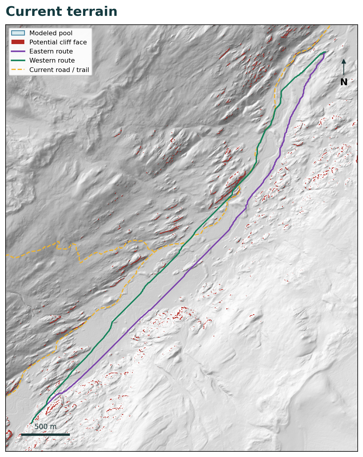
The easiest route can use the broad valley floor.
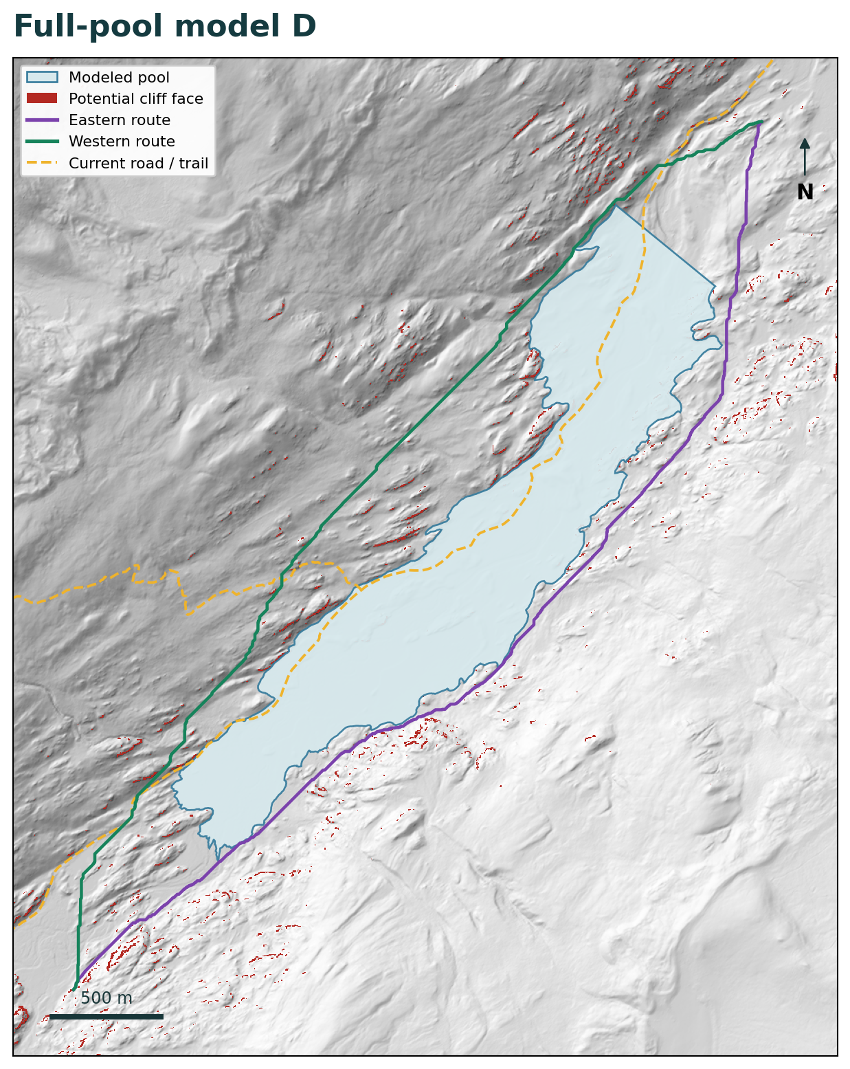
The modeled water occupies the central corridor and pushes routes onto the slopes.
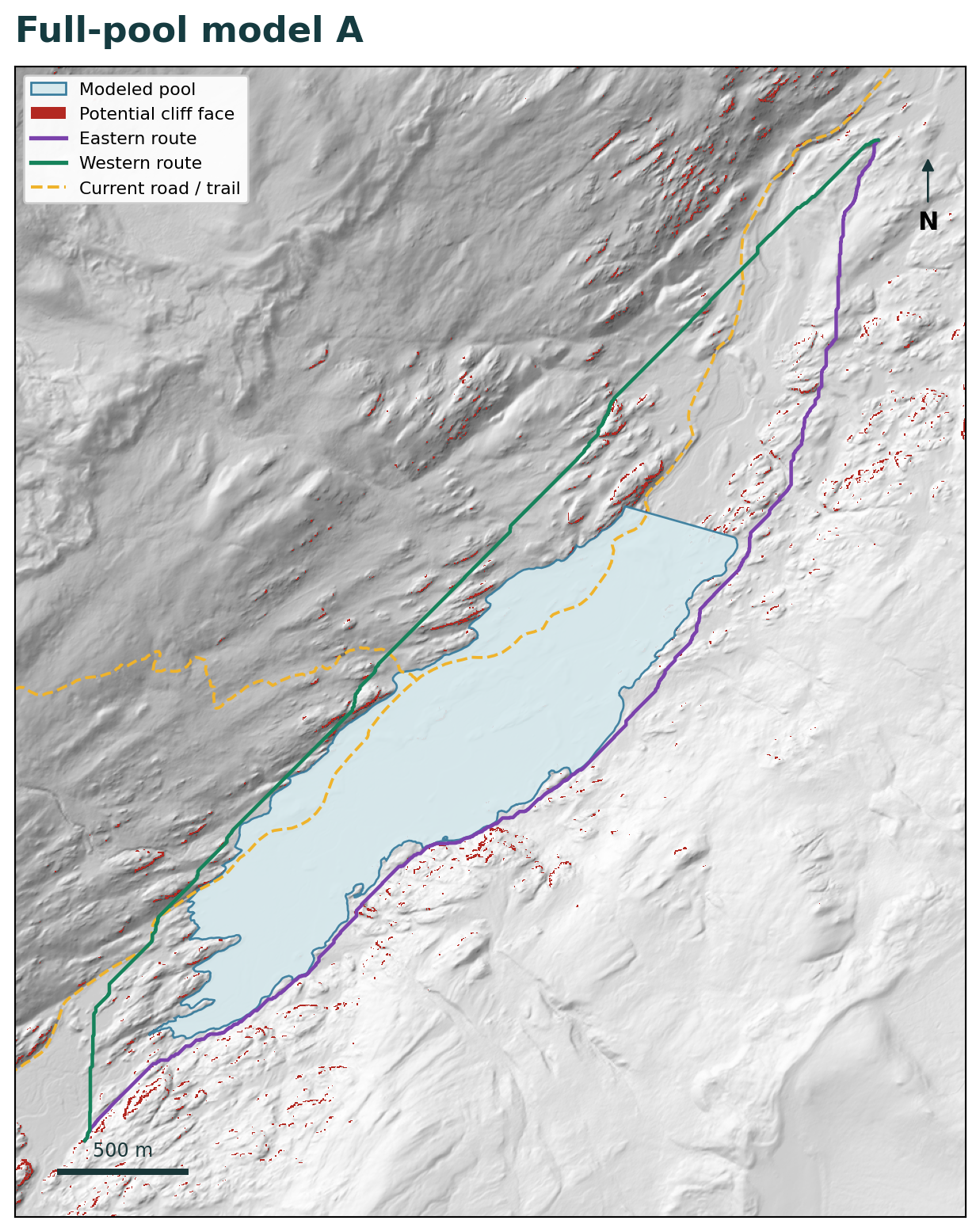
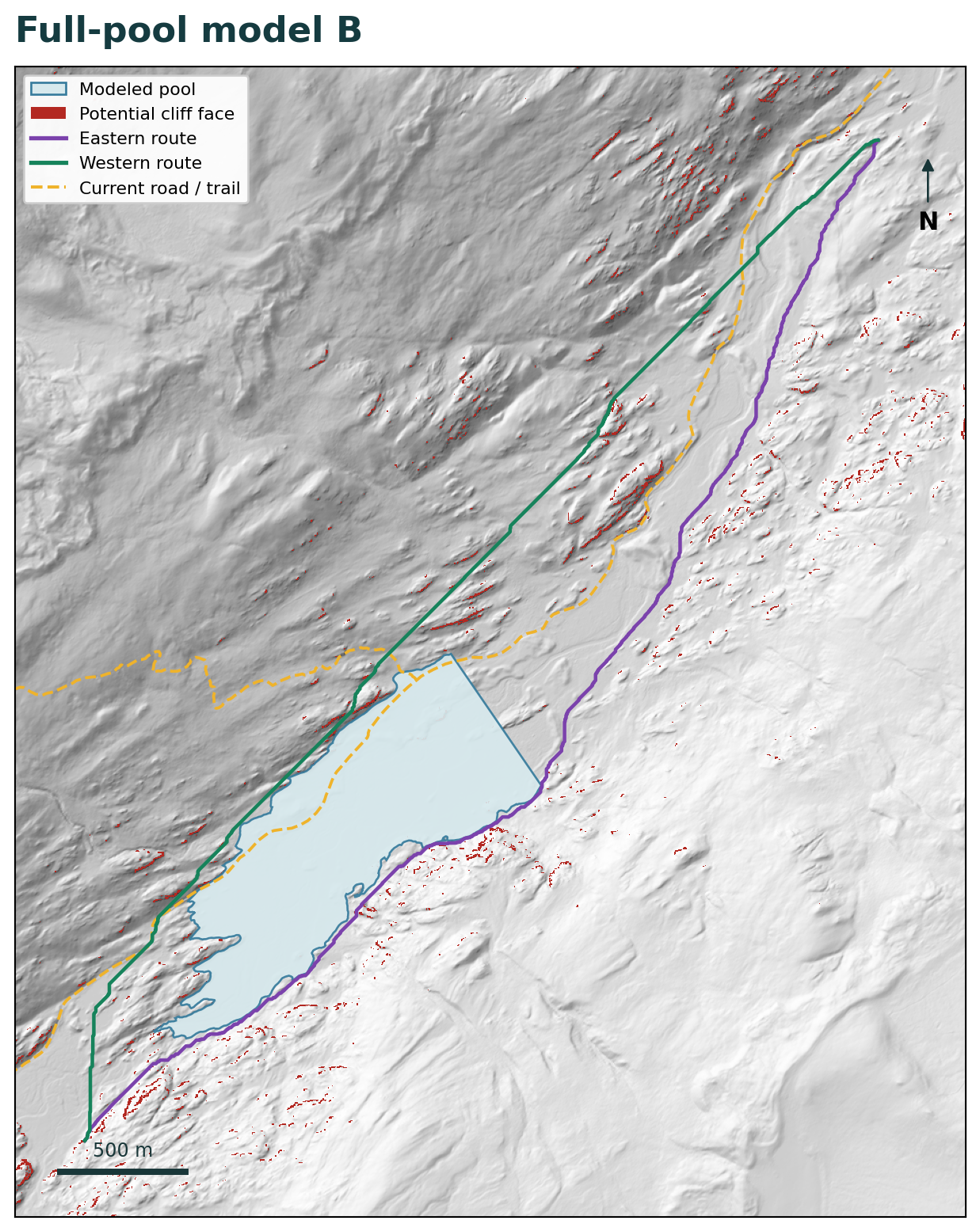
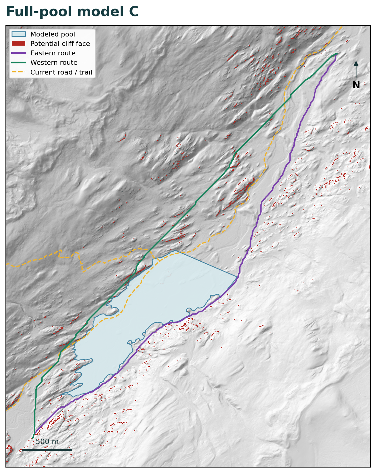
All maps use the same central gates and the primary 2 metre terrain rules. The lines show computational routes, not observed animal tracks.
Calculation method
The details below show how the terrain routes were compared and where the numbers in the maps came from.
The source is the georeferenced 2016 USGS lidar-derived 1 metre bare-earth digital terrain model. The analysis domain is 5,800 by 5,700 metres with a 100 metre source halo. Coordinates use EPSG:32613, with bounds of easting 376,000 to 381,800 metres and northing 4,362,500 to 4,368,200 metres.
Modeled pools and existing ponds are barriers. Their polygons are expanded by half a routing-cell diagonal before cell centers are tested. Existing mapped streams remain traversable under the crossing and fording assumption used in the earlier analysis.
The main route model excludes broad hillsides steeper than 35 degrees. That broad slope is calculated from the mean 10 metre terrain with a 20 metre central-difference span, then interpolated to the 2 metre routing grid.
A 1 metre cell is classified as a candidate steep face only when it meets both tests:
A 2 metre route cell is blocked when any of its four underlying 1 metre cells meets both tests. The classifier adds no gap closing, dilation, component pruning, or modeled rockfall runout.
Each traversable cell connects to as many as eight neighbors. A diagonal move is allowed only when both adjoining orthogonal cells are also open, preventing a route from cutting between two blocked corners.
Each directed edge costs its 3D length multiplied by the normalized anisotropic routing cost from Berti et al. (2022):
r(θ) = [8.303 + exp(3.17 + 0.0002θ² + 0.003θ)] / [8.303 + exp(3.17)]
θ is the signed grade of movement in degrees, so uphill and downhill travel receive different costs. Results are relative terrain-effort units rather than calories or a species-specific probability of passage.
An implicit C++ A* solver calculates neighbors as needed. Its lower-bound heuristic uses the global minimum cost multiplier, reached at a 7.5 degree descent, multiplied by straight-line horizontal distance to the destination gate. Independent tests compare A*, full Dijkstra, and reverse-edge distances against a separately built SciPy graph.
The opportunity envelopes answer a different question from the single easiest route: how much terrain remains available if a route may cost slightly more than today's minimum?
Full Dijkstra accumulation calculates the minimum cost from the upstream gate to every cell. A reversed-edge calculation does the same from every cell to the downstream gate. Adding those two values gives the minimum possible gate-to-gate cost of a route that passes through each cell.
Every alternative is then tested against the same current-valley minimum multiplied by 1.05, 1.10, and 1.20. The reported between-gate area includes cells within northings 4,363,455 to 4,367,455 metres that remain inside each shared cost budget.
Writing the rule explicitly: C(v) = d(upstream, v) + d(v, downstream). A cell is eligible when C(v) ≤ (1 + b) × C₀, where C₀ is the current-valley minimum and b is 0.05, 0.10, or 0.20. For example, the current minimum of 5,325.3486 relative-cost units gives a +5% ceiling of 5,591.6160 units. Eligible 2 by 2 metre cells inside the between-gate band contribute 4 square metres each; the reported loss is 100 × (A₀ − Aₛ) / A₀, using the same budget for the current and reservoir scenarios.
| Scenario | Purpose |
|---|---|
lidar-source 10 m | Averages the lidar terrain to 10 metres while retaining the 35 degree broad-slope ceiling, original gates, and original separator. This isolates the change in terrain source. |
fine 2 m-no-cliff | Uses native 2 metre routing elevations with the same broad 10 metre-supported slope screen, but without the candidate steep-face mask. |
fine 2 m-primary-cliff | Adds the primary 1 metre candidate steep-face mask while retaining the same terrain, water, gates, and costs. Its paired difference isolates the mask's effect. |
cliff 45 / cliff 70 | Changes only the candidate-face slope threshold. |
cliff 60-span 4 | Keeps the 60 degree threshold but increases the fine-slope derivative span from 2 to 4 metres. |
primary-cliff-shoreplus 10 | Adds a 10 metre outward expansion to each modeled pool as a shoreline-position sensitivity. |
primary-cliff-quiet 250 | Excludes cells within 250 metres of the same current road and trail alignment in both the baseline and reservoir comparisons. |
native 2 m-slope 35 | Applies the 35 degree ceiling from the native 2 metre grid instead of the broader 10 metre-supported slope. |
The central cases test either-side, east-side, and west-side routes in both directions. Additional sensitivities test either-side and east-side routes, with the 250 metre quiet scenario using either side. Together they produce 200 directional route records.
effort_change_pctadded_cliff_effort_pctascent_native_mascent_smooth_10_maccess_within_100_m / 250_mnewly_excluded_cliff_cells_before_sideOpportunity-envelope area is a computational measure of route choice within a common terrain-cost budget. It is distinct from occupied habitat acreage or a measured biological corridor width.
g++ -O3 -std=c++17 scripts/implicit_astar.cpp -o scripts/implicit_astar.python3 scripts/run_lidar.py to recreate all 200 route records.python3 scripts/compute_envelopes.py to recreate the 5%, 10%, and 20% route-opportunity summaries.The independent review reconstructed all 200 exported paths, checked 375,693 vertices and 256,431 diagonal edges against the saved constraints, recalculated route metrics, and found no numerical defect in the reviewed implementation or final outputs.
Required Python packages are NumPy, SciPy, Shapely, PyProj, and Rasterio. The saved package retains the source terrain, masks, routes, results, scripts, environment record, and checksums needed to reproduce the analysis without new data retrieval.
How to read the result
The reservoir-driven detour is the main modeled change. In matched runs, adding the primary candidate steep-face mask changes route cost by no more than 0.0292%. The mask shows where the displaced route meets locally abrupt terrain, while the calculation keeps animal behavior, vegetation, snow, footing, fencing, construction disturbance, and future road changes outside the model.
Every tested route remained mathematically connected. The important change is what that connection requires: more climbing, higher terrain cost, and substantially less low-cost room to choose another path.
Open evidence
Analysis completed September 24, 2026. Lidar acquisition: 2016. Addendum 2.0.